
This post is an adaptation of a paper that I wrote to answer the question of what is the best way to value draft picks in trades. The original paper can be found here in its intended format. Converting this to a blog post led to some difficulties in formatting, especially when it comes to captions on multi-figures, but I hope it is as clear as possible.
I. Introduction
Draft picks are an important commodity in the NBA, able to be used to directly add players to a team, or they can be traded as assets for current players, other draft picks, or other assets. Therefore it is important to be able to place a value on those draft picks in an abstract sense. As with everything in the NBA, how well one is able to do that depends entirely on the situation, however it is possible to make assessments based on generic situations, and then to allow the actual circumstances to dictate the final decision.
This paper will be concerned with assessing the value of draft picks in prospective trades; it will consider the generic case of a team trading the rights to a future draft pick given certain protections, finding the probability of where the pick should be expected to fall based on the team’s performance and projections for the future, and giving a relative value to each drafting position. There is a bit of feedback in this situation, because accurately projecting how well a team will do depends on being able to predict how much the rookies on the team will help them, but that will be accounted for.
In the end, the goal is to have a function that will be able to provide the expected value of a team’s future draft pick, taking into account any protections placed on the pick, as well as the likelihood that it will be transferred (i.e. not protected) in the nearest draft.
In Section II, I will cover some of the basic rules for the draft, focusing mainly on the lottery system. In Section III, I will describe how to find a mapping of a team’s winning percentage onto their likely finishing position in the league that season. From there, I will describe how to determine the drafting order based on a team’s likely finishing position in Section IV. Then in Section V, I will describe how to come up with a way to give a value to each pick in the draft, from 1 to 60, based on past performance of players picked in each position. In Section VI, a number of methods will be presented to predict a team’s winning percentage at the end of the season that leads into the draft. Finally, in Section VII, I will put all of the parts together to form a cohesive way of evaluating a team’s draft pick for the purposes of a trade.
II. Drafting Rules
Draft ordering is separated into two sets of teams: those who make the playoffs; and those who miss the playoffs. Currently (since 2005), there are 30 teams in the NBA, 16 of which make the playoffs (the top 8 from each conference), and 14 (7 from each conference) who miss the playoffs. The teams which make the playoffs are given picks 15-30 in order of worst final winning percentage, thus the team with the best winning percentage will pick last; performance in the playoffs does not matter for draft seeding. Teams with the same winning percentages utilize a coin toss to determine ordering for the first round; that ordering changes in the second round. The teams which miss the playoffs are entered into a lottery to determine the 1-14 draft ordering.
The odds for the lottery are given based on finishing order, where the team with the worst record gets the best odds, and they decrease after that, falling off faster than exponential decay. The team with the worst record in the previous season has a 25% chance of getting the first pick, while the team with the best record that missed the playoffs has only a 0.5% chance. Once a team wins the number 1 draft spot, they cannot win the number 2 or 3 spots, and so the odds change for the number 2 and 3 picks, but they are all based off of these initial odds. Once the lottery teams have been selected, the remaining teams are seeded in order of worst finishing record. Thus the team with the worst record in the league can drop only as far as the $latex 4^{th}$ spot. Table I lists the odds for a team in each finishing order winning any of the 14 draft positions, and Figure 1 shows the chances each position has of receiving the first pick. [Wikipedia]
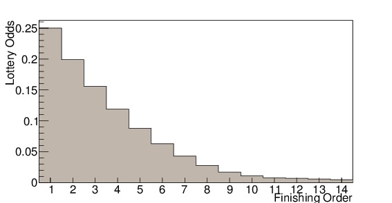
Figure 1. Lottery odds by finishing order for the previous season. The fall off is slightly faster than an exponential decay.
Draft picks are able to be traded between teams for players, coaches, other draft picks, and to some extent money. The teams are allowed to put restrictions on the transferring of the pick, such that if the pick falls in a certain range of draft positions, the pick will not be given that year, and other provisions are made, generally resulting in a pick in the next draft, with its own set of restrictions. Up to 55 draft slots may be protected in this way in a particular draft. Draft picks count as $0 for salary cap purposes until they are signed. Draft picks may be traded up to 7 years in the future. There are also certain other rules that apply, such as teams not being allowed to trade their first-round draft pick for consecutive seasons, but they are beyond the scope of this paper. [cbafaq.com/salarycap.htm]
Note that all assessments of the draft made in this paper will assume that the draft follows this set of rules, and that there are no special circumstances in the upcoming draft; an example of a special circumstance would be an expansion team joining the league and being guaranteed a top-3 pick.
| fo | Draft Order | |||||||||||||
|---|---|---|---|---|---|---|---|---|---|---|---|---|---|---|
| 1 | 2 | 3 | 4 | 5 | 6 | 7 | 8 | 9 | 10 | 11 | 12 | 13 | 14 | |
| 1 | 0.250 | 0.215 | 0.178 | 0.357 | — | — | — | — | — | — | — | — | — | — |
| 2 | 0.199 | 0.188 | 0.171 | 0.319 | 0.123 | — | — | — | — | — | — | — | — | — |
| 3 | 0.156 | 0.157 | 0.156 | 0.226 | 0.265 | 0.040 | — | — | — | — | — | — | — | — |
| 4 | 0.119 | 0.126 | 0.133 | 0.099 | 0.351 | 0.160 | 0.012 | — | — | — | — | — | — | — |
| 5 | 0.088 | 0.097 | 0.107 | — | 0.261 | 0.360 | 0.084 | 0.004 | — | — | — | — | — | — |
| 6 | 0.063 | 0.071 | 0.081 | — | — | 0.439 | 0.305 | 0.040 | 0.001 | — | — | — | — | — |
| 7 | 0.043 | 0.049 | 0.058 | — | — | — | 0.599 | 0.232 | 0.018 | — | — | — | — | — |
| 8 | 0.028 | 0.033 | 0.039 | — | — | — | — | 0.724 | 0.168 | 0.008 | — | — | — | — |
| 9 | 0.017 | 0.020 | 0.024 | — | — | — | — | — | 0.813 | 0.122 | 0.004 | — | — | — |
| 10 | 0.011 | 0.013 | 0.016 | — | — | — | — | — | — | 0.870 | 0.089 | 0.002 | — | — |
| 11 | 0.008 | 0.009 | 0.012 | — | — | — | — | — | — | — | 0.907 | 0.063 | 0.001 | — |
| 12 | 0.007 | 0.008 | 0.010 | — | — | — | — | — | — | — | — | 0.935 | 0.039 | — |
| 13 | 0.006 | 0.007 | 0.009 | — | — | — | — | — | — | — | — | — | 0.960 | 0.018 |
| 14 | 0.005 | 0.006 | 0.007 | — | — | — | — | — | — | — | — | — | — | 0.982 |
Table I. The odds of ending up in a given Draft Position based on finishing order, fo, among the lottery teams. Dashes indicate zero probability of getting that position. (Source: Wikipedia)
III. Mapping Winning Percentages onto Final League Ordering
The first step to determining which draft pick a given team will have in an upcoming draft is to come up with a mapping of winning percentages onto finishing order with respect to the other teams in the league. From there, it is a simple calculation to get the odds of the pick landing in any given position.
The final ordering of teams in terms of lottery odds and playoff teams will change from year to year based on how the wins are distributed, but for the most part, knowing a team’s winning percentage at the end of the season will allow one to determine each team’s ordering to within a few spots. In order to find this mapping, I first binned the data by winning percentage. I chose to use the 2005-2014 seasons as the data from which to build the map, since 2005 was the first season in which there were the current number of 30 teams in the league.
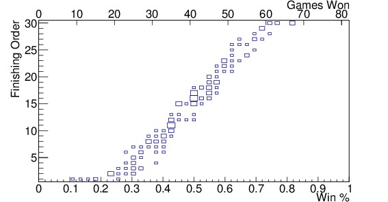
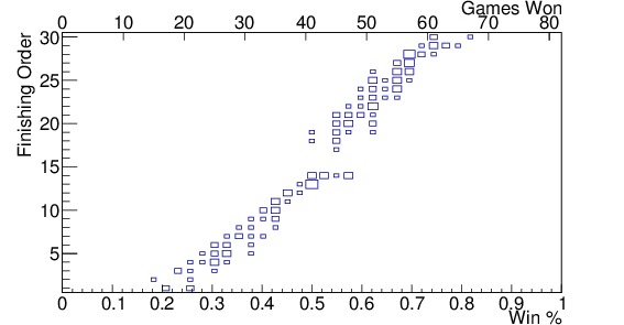
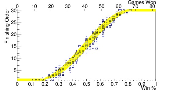
Since there are 82 games in a normal NBA season (some seasons are shorter due to strikes or lockouts — 2012 for example), and there are 30 teams each season over 10 years (since 2005), a bin size of 2 wins (corresponding to $latex 2/82 sim 0.024$ in winning percentage) seems appropriate. Figure 2 shows the results of such a binning for (a) teams in the Eastern Conference, (b) teams in the Western Conference, and (c) all teams in the league. The analysis done here will consider all teams in the league, instead of the two conferences separately, but it is important to see that there is a distinction between the two conferences for teams winning between 40 and 50 games. In the Western Conference, those teams are more likely to miss the playoffs than similar teams in the East. For each of the past 10 years, the three teams with the worst records among the playoff teams have been from the Eastern Conference, with one exception. This balance of power is likely to change at some point in the future, but the conference of the team being traded with should be considered for now.
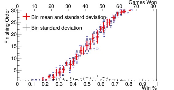
Once the data were binned, I found the mean and standard deviation of both the finishing order and winning percentage in each bin. Figure 2 (c) shows the mean and standard deviation for each bin overlain on the distribution. I then fit the resulting set of points. Since data take the shape of an S, a third-order polynomial is a good approximation, at least in the range where most of the teams fall — from a winning percentage of 0.2 to 0.8. The size of the standard deviation of each bin can be approximated by a second-order polynomial between winning percentages of 0.2 and 0.8. Once the functions for the mean and standard deviation have been found, it is a simple matter to find the likely finishing order for any team from their winning percentage. Figure 2 (d) shows the resulting function, which I will call $latex F(p)$, as a yellow band, where the width of the band indicates the standard deviation, $latex sigma_F(p)$, expected. The actual results are overlain to show the agreement. Note that below a winning percentage of 0.2, we have assigned a mean of 1 and standard deviation of 0.5, as all teams below 17 wins have had the worst record in the league for that season. Similarly, teams with a winning percentage above 0.8 are given the $latex 30^{th}$ slot with a standard deviation of 0.5, because all teams with more than 65 wins in a season have had the best record in the league for that season.
(a)
(b)
(c)
(d)
Figure 2. Finishing order vs winning percentage since 2005 for (a) teams in the Eastern Conference, (b) teams in the Western Conference, (c) all teams in the league along with the mean and standard deviation for each bin shown in red, and the standard deviations by themselves shown in black along the bottom, and (d) shows all teams in the league as well, but with the fit function, $latex F(p)$, shown in the yellow band; the size of the band indicates the standard deviation, $latex sigma_F(p)$. The axis at the top indicates the number of games won in an 82-game season corresponding to that winning percentage. The 2012 strike-shortened season was included. Note the gap in finishing order distribution in the Western Conference from 15-17. This indicates that teams in the Western Conference are more likely to miss the playoffs, and thus be in the lottery, with a higher winning percentage, than teams in the Eastern Conference.
IV. Drafting Position Probabilities
Next, the probability of a team with a given winning percentage and standard deviation landing in any particular draft position must be calculated. Teams are awarded two draft slots per season, one in the first round and one in the second round. The first-round slots are awarded based on the lottery results, and then playoff teams, while the second-round slots ignore the lottery ordering and simply go based on finishing order for the two groups, except that in cases of ties between winning percentages, the positions get flipped between rounds. In order to get the probability for each slot, it is necessary to first calculate the probability of ending the season with a given winning percentage, the probability of that winning percentage turning into each position in overall finishing order, and then the probability of that finishing order changing with the lottery.
The probability, $latex mathcal{P}_{wp}(p)$, of the team ending the season with a given number of wins, w, after playing n games, corresponding to a winning percentage of $latex p = w/n$, can be calculated using Gaussian probability once a predicted winning percentage, $latex P$, and standard deviation, $latex sigma_P$ have been provided. The probability is given by
$latex mathcal{P}_{wp}(w,n|P,sigma_P) = frac{1}{nsigma_Psqrt{2pi}}e^{-frac{(p-P)^2}{2sigma_P^2}}.hfill(1) &s=2$
Likewise, the probability, $latex mathcal{P}_{fo}(f|p)$, of a team ending up in a given position, $latex f$, in the finishing order of all teams in the league, given that they finished with a winning percentage of p, can be written as
$latex mathcal{P}_{fo}(f|p) = frac{1}{sigma_{F}(p)sqrt{2pi}}e^{-frac{(f-F(p))^2}{2sigma_{F}(p)^2}}.hfill(2) &s=2$
where $latex F$ and $latex sigma_{F}$ are the mean of the predicted finishing order and its standard deviation, which are functions of p, calculated in Section III.
The probability of getting a particular draft spot given a particular finishing place, $latex mathcal{P}_{do}(delta|f)$, then depends on the lottery. If the team is not in the lottery, then their draft position, $latex delta$, equals their finishing order; if they are in the lottery, then their draft position is a discrete function of the finishing order, $latex g(f,delta)$, able to be read off of Table I; so the equation can be written piece-wise as
$latex mathcal{P}_{do}(delta|f) =
begin{cases}
g(f,delta) & ~~~~~~~~~~~~~ text{(lottery)} \ hline
1 & text{if } delta = f ~~~ text{(non-lottery)} \
0 & text{if } delta neq f ~~~ text{(non-lottery).}
end{cases}hfill (3)
$
The total probability for each draft spot, given the predicted winning percentage, $latex P$, and standard deviation $latex sigma_P$, can be written as $latex mathcal{P}(delta|P,sigma_P)$, and is the sum over the probabilities for all possible ways that slot could be obtained, which is given by
$latex mathcal{P}(delta|P,sigma_P) = sumlimits_{f = 1}^{30} [mathcal{P}_{do}(~delta|f) timessumlimits_{w=1}^{n}(mathcal{P}_{wp}(w,n|P,sigma_P)timesmathcal{P}_{f}(f|p))] .hfill (4) &s=1$
Thus, once a prediction has been made for the team’s winning percentage and standard deviation, the probability for that team getting each draft slot can be predicted using Equation (4).
A. Examples
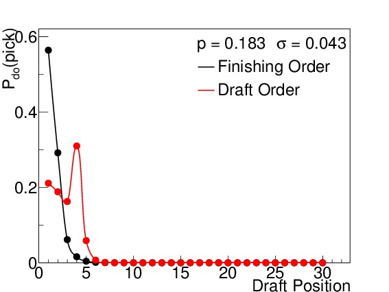
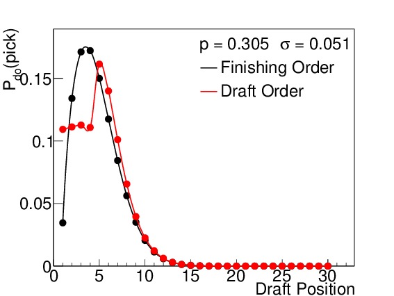
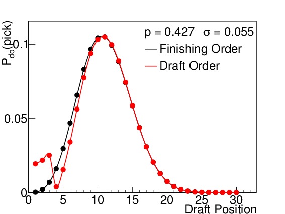
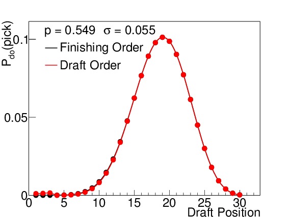
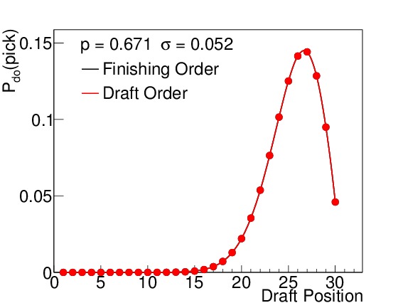
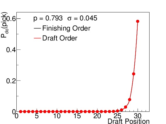
By way of example, I calculated the odds both for finishing order (which is relevant for the second-round ordering) and first-round drafting order. Figure 3 shows these probabilities for six different winning percentages, which correspond to 15, 25, 35, 45, 55, and 65 wins respectively (when n=82). I elected to use the binomial standard deviations (see Equation (5)) to illustrate how spread out the results are even under the absolutely best circumstances possible (prior to the season) even though such precision is not practically realizable. Teams with non-zero probabilities of finishing in spots 1-14 will be affected by the lottery, but to varying degrees. The teams with 15-45 wins each have scenarios in which they finish in the lottery, but the effects of the lottery odds are much stronger on the teams with 15, 25, and 35 wins than on the team with 45 wins, where the difference is almost imperceptible. Teams finishing with 55 or more wins are completely unaffected by the lottery, but still show a wide variety of places they can finish with respect to the league.
(a) 15 wins
(b) 25 wins
(c) 35 wins
(d) 45 wins
(e) 55 wins
(f) 65 wins
Figure 3. $latex mathcal{P}_{do}(pick)$ for all 30 draft positions for a win total of (a) 15, (b) 25, (c) 35, (d) 45, (e) 55, and (f) 65, assuming a binomial standard deviation. The black points indicate the probability for finishing in that place in the league (and drafting order for the second round), while the red points indicate the probability for drafting in that position in the first round. Above draft position = 14, the two are always identical. The team with 15 wins has an almost 60% chance of being the worst team in the league, but its most likely drafting position in the first round is number 4, due to the lottery. The teams with 25 and 35 wins also have their odds of picking 1-14 slightly altered. The team with 45 wins has a barely perceptible difference between his finishing order odds and draft order odds for low draft picks. The teams with 55 and 65 wins are completely out of the lottery, and so their two odds are the same. Note that these standard deviations are the best we could ever conceivably do (prior to the season), and there is still a wide range of possible draft positions for each team.
V. Valuing Draft Picks
Ultimately, the value of a draft pick depends on what a team does with it. Teams can trade the pick before they even receive it, trade it before or during the draft, or they can use the selection on a player, and then they can sign him, trade him, or release him. One team may use a pick on the exact player needed to fill a certain role on the team, others choose the best player available, still others draft players already playing in foreign leagues, who won’t play in the NBA for some time. Each of these teams may be valuing their pick differently.
Generally speaking, the value of the pick is related to the quality of player that can be obtained with the pick, and the number of options available to the team. Thus, the number 1 pick in the draft will always be very desirable because the team with that pick has the maximum number of choices, and in theory that team can always get the best player (at least for their own purposes). But how much less valuable is the second pick than the first, and then how much less is the third, fifth, tenth, etc?
The main goal an NBA team is of course to win games and championships, and make money while doing so. Thus, there are at least two ways to consider how much a player is worth to his team: how many games/championships he can win; andhow much money he can make for the team over his own salary. To some extent, the NBA has already placed a valuation on the draft picks by means of the rookie pay scale. This specifies a salary to each draft position, and whatever team signs that player (whether he was drafted by them, or his rights were traded after the draft but before signing) must pay him that salary to within 20%. The relative pay scale can be seen in Figure 4. There are mandatory raises after each of the first two seasons, but the ratio stays the same. Once a player reaches his fourth year, the inequality starts to change. For the most part, players in their first five years should be considered a bargain compared to the cost of a free-agent providing the same minutes and statistics. Also, any attempt to quantify how much money a generic player could earn for his team would be directly tied to the stats I will look at. As a result, I have elected not to consider the draft pick’s potential salary, or the monetary value he can bring to the team in this study. [cbafaq.com/salarycap.htm]
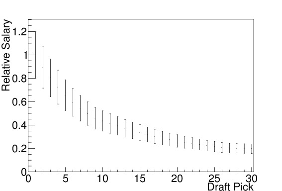
Figure 4. The rookie pay scale, shown with salaries relative to the number 1 draft pick. The bars indicate the range in salary that may be offered to the player.
I won’t go into all the details of rookie contracts here, but the basic gist is that teams have the rights, or at least options to the rights, to a player they drafted for the first four years of his career, with additional rights to contract offers for the fifth; after that they become free-agents to some extent. Players certainly may stay with the team that drafted them after that point, but they are not obligated to. Therefore it makes sense to consider a player’s worth in his first five seasons in the league, which may or may not start the season after he was drafted. [cbafaq.com/salarycap.htm]
There are many ways in a which a player may be considered valuable to his team, some players might score a lot of points, others might grab a ton of rebounds, another may be a skilled defender, and a last one may be able to give his team 45 minutes a night. So how to quantify the value of a particular draft position, when players of many different styles may have been chosen in that spot? Using points, or rebounds, or field-goal percentage will not properly quantify the player, because players from different positions generate stats at differing rates. In my mind there are two things that should factor above any particular statistics, did the player help his team win games, and how much time was he out there helping his team win games?
Win shares are a statistic based off of Bill James work in baseball, and are calculated and tabulated by Basketball-Reference.com. This stat takes into account both offensive and defensive contributions to the team by each player, and tries to determine how responsible he was for his team winning the games they did. I am still a little bit skeptical of this statistic because I have not calculated it myself and have no way to ascribe an uncertainty to it, but it does a reasonable job of determining how important players are with respect to others, and I think it accurately encapsulates how many wins a player brought to his team (as will be seen later). But additionally, we should consider how much time the player is on the court for his team in those 5 years; for some teams, simply having a player who can produce a lot of minutes even if it is not of the highest quality, is important.
It is necessary to calculate the average and standard deviation of the number of win shares and minutes played by all players chosen in each of the first 60 spots of the draft (i.e. the first two rounds), both in the first five years of their career, as well as just the first season. The need to look at just the first year is because we need to be able to add these rookies expected win shares and minutes played to their teams’ rosters for their next season, as will be used in Section VI.
Using the seasonal stats for every player drafted from 1985-2013 (players drafted in 2014 cannot be evaluated yet), I separated players based on their draft position. For players in the 1980s, when there were more than two rounds, I decided to make a hard cut at the end of the second round. This means that the last few picks only have a few players because there have only been 30 teams since 2005. For the first-year stats, all years between 1986 and 2014 were used for performance, but for the five-year stats I only look at players who started their careers in 2009 or before, so that they had a full five seasons in the league. If a player was drafted, but did not play his first season until a few years later, his five-year clock starts with his first game played. This may be inaccurate contract-wise with certain players, but it is generally correct. There are many players who were drafted and never played in the league for various reasons; their null stats are included because it helps to show the lower performance of some of the later picks.
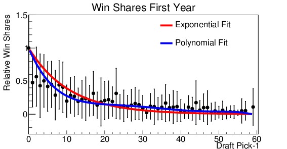
(a)
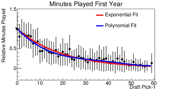
(b)
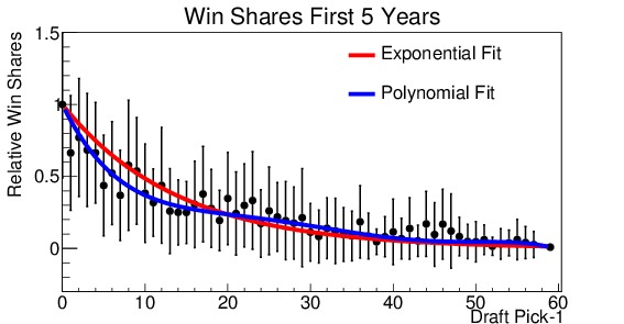
(c)
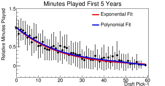
(d)
Figure 5. Relative analysis of draft picks performance for (a) win shares during his first year in the league, (b) minutes played during his first year, (c) win shares during his first 5 years in the league, (d) minutes played during his first 5 years in the league. Everyone is measured with respect to the number 1 draft pick. Note that the x-axis is shifted down by 1, so that the number 1 pick becomes the number 0 pick (for ease in fitting). Two fit lines are shown for each, the first an exponential decay and the second a fifth order polynomial.
Figure 5 shows the four distributions. They are shown on a scale relative to the number 1 draft pick. Also note that the x-axis has been shifted such that the number 1 pick is shown at 0, this is for ease in fitting the distribution. It is readily apparent from all four graphs that there is a marked fall-off after the number 1 pick. By the tenth pick, performance has already dropped to approximately half of that of the top pick. Now, various fit functions can be used to describe the distribution. The decay appears to be exponential, so each is fit with an exponential function (shown in red on the plots). For the number of minutes played, the exponential fit is excellent. However, for win shares the fit tends to over-estimate players drafted in the 3-20 slots, and under-estimate the later picks. So I used a fifth-order polynomial to obtain a better fit. This fit is shown in blue on the plots. The difference between the two fits is small for the minutes played, but much more significant for the win shares. The polynomial fit produces a much better $latex chi^2$ result, indicating a better fit. The polynomial fit will be used to make projections.
This is, of course, a fairly simple model, worrying only about the win shares produced and minutes played. However, in the generic case of evaluating draft picks, it seems appropriate. If a team has a specific need or situation, this data can be looked at in another way. For instance, consider the 2007 draft when Greg Oden and Kevin Durant were each available; the team with the number 1 draft spot that year (Portland) might want to look at the performance of centers vs shooting guards/small forwards, consider the possibility for injury with players from both positions, etc. Of course, any statistic could be used for evaluation purposes here, points, total points produced, rebounds, etc; and the players used in the analysis can be a subset of the total number, (e.g. looking at players by position); whatever the team needs can be analyzed draft pick by draft pick in this manner.
VI. Predicting a Team’s Winning Percentage
Now that the mapping of winning percentages onto final ordering and draft ordering has been determined, and the value of the draft picks has been set, it is necessary to be able to predict a team’s winning percentage at the end of the season. This is a tall task. There is a limit to how well any prediction can be made. Even if an incredibly accurate prediction could be made about each teams’ skill level at any point before or during the season, random statistical fluctuations do no allow you to make predictions to better than within about 5 games on average, and that’s assuming that the team’s skill level (as well as the skill levels of all the other teams in the league) does not change, which it certainly will, due to injuries, trades, free-agent signings, rookies being an unsure commodity, etc. Taking these as caveats, it is still possible to come up with predictions in a reasonable manner.
It will be assumed throughout this section that predictions are being made between seasons, and that all the stats from the previous season are available. If it is close enough to the start of the next season that a reasonable approximation of the team rosters exists, then better predictions can be made. If predictions are being made after $latex n$ games in the current season, the current winning percentage, $latex p$, can be used as a prediction for the rest of the season, with a standard deviation of
$latex sigma = sqrt{frac{p(1-p)}{n}}.hfill (5) &s=2$
Predictions from the start of the season can be combined with the in-season results by means of a weighted average, using the standard deviations, $latex sigma_i$, of each of the predictions as the weights, by means of
$latex p_{weighted} = frac{frac{1}{sigma_1^2}p_1 + frac{1}{sigma_2^2}p_2}{frac{1}{sigma_1^2} + frac{1}{sigma_2^2}} . hfill (6) &s=2$
The standard deviation on that prediction is given by
$latex sigma_{weighted} = frac{1}{sqrt{frac{1}{sigma_1^2}+frac{1}{sigma_2^2}}}.hfill (7) &s=2$
Note that these predictions would be good for the remainder of the current season. Thus, to come up with the final prediction you need to combine the two predictions as
$latex p_{final} = frac{np + (n_{tot}-n)p_{weighted}}{n_{tot}}, hfill (8) &s=2$
where $latex n_{tot}$ is the total number of games in the season, generally 82,but sometimes less.
Alternatively, a method could be developed to predict results at the end of the season based on statistics generated from the on-going season, such as current winning-percentage, etc; but such a method will not be developed in this section. See the conclusion for descriptions of how the methods developed in this section can be adapted for mid-season predictions.
There are many ways to predict a team’s winning percentage in the coming season. We will look at a few such ways below, discussing their method and formulation, as well as strengths and weaknesses.
A. League Average
The absolute easiest prediction that can be made is simply to assume every team will win the league average number of games — that is, exactly half — with a standard deviation given by the standard deviation in the winning percentages in the previous year. This prediction uses no information about the teams, and treats each of them equally, and therefore is a weak tool. However, it will be useful to compare other methods to this one, so this will be used as a baseline test.
B. Last Year’s Winning Percentage
The next easiest prediction is simply to use the team’s performance from the previous season as the guess. Thus, the winning percentage from last year is the guess, and the standard deviation is obtained from Equation (5). This prediction does treat each team differently, however, it assumes that the team does not change in the off-season, which it certainly will, adding and subtracting players, changing coaches and styles, etc. This method will also mostly be useful as a means of comparison.
C. Similarity Methods
A better prediction can be made by using the team’s statistics. A number of teams similar to the team in question can be found from previous NBA seasons using some metric, and then those teams’ performances in the season immediately following that one can be used to come up with a prediction and standard deviation. This method relies on a distance metric, which I have described in both of my previous papers. In this case, we define the distance metric as
$latex d_{ij}^2 = sumlimits_{k=1}^4 w_k(frac{s_k^i-bar{s}_k^{i,pop}}{sigma_k^{i,pop}} – frac{s_k^j-bar{s}_k^{j,pop}}{sigma_k^{j,pop}})^2, hfill (9) &s=2$
where $latex d_{ij}$ is the distance between seasons i and j, with season i being the season in question; the $latex s_k$ are the statistics we will be using; $latex bar{s}_k^{i,pop}$ is the mean of $latex s_k$ for the population from which season i was drawn (i.e. if season i is from the 2014 season, then $latex bar{s}_k^{i,pop}$ is the mean of $latex s_k$ for all teams in the 2014 season); $latex sigma_k^{i,pop}$ is likewise the standard deviation for the population from which season i was drawn; and the $latex w_k$ are the weights assigned to those statistics.
Equation (9) can be used with any number of different statistics, so long as they have well-defined means and standard deviations. Given a season that you would like to find the N most similar seasons for, it is only necessary to search through all the possible team-seasons available (this may be limited depending on the objective) and calculate $latex d_{ij}$ for each pair, and select the N closest. The number N will be significantly smaller here than it is when looking at players because the number of teams is much smaller. N is chosen to be 10 unless otherwise noted. Once the N teams have been selected, it is simply necessary to get the average and standard deviation of their next season results.
For example, if the 10 most similar teams have the following results for number of wins in their next season, [50, 52, 60, 45, 58, 41, 55, 51, 38, 51], and they were all played in 82-game seasons, then the predicted winning percentage is 0.611, about 50 games, and the standard deviation is 0.085, or about 7 games.
i. Same Team Last Season
One set of statistics that can be used to determine similarity is the set of four factors, identified by Dean Oliver as the keys to success in basketball, for the team in the previous season. These factors are a team’s offensive-rebounding percentage, effective field-goal percentage, offensive-turnover percentage, and free-throw-made rate. Additionally, their defensive counterparts should be considered as well. Thus, the combined offensive-rebounding percentage that their opponents had in games against them, as well as the other three stats, should also be considered.
To be clear on the calculation of the four stats, I list their formulas below:
$latex orp = frac{orb}{orb + drb_{opp}} hfill (10) &s=2$
is the offensive-rebounding percentage, where orb is the number of offensive rebounds, and $latex drb_{opp}$ is the number of defensive rebounds that their opponents grabbed;
$latex efgp = frac{fgm + 0.5cdot threem}{fga} hfill (11) &s=2$
is the effective field-goal percentage, where fgm is the number of field-goals made, threem is the number of three-point field-goals made, and fga is the number of field-goals attempted;
$latex top = frac{tov}{poss} hfill (12) &s=2$
is the turnover percentage, where tov is the number of turnovers, and poss is the number of possessions, where
$latex poss = fga + tov + 0.44 cdot fta – orb~, hfill (13) &s=2$
and fta is the number of free-throws attempted; and finally
$latex ftmr = frac{ftm}{fga} hfill (14) &s=2$
is the free-throw-made rate, where ftm is the number of free-throws made.
In addition to these eight stats (four offensive, four defensive), we also include the team’s winning percentage in the preceding season. The relative weighting of these nine factors was determined based on fitting, however, I will not go into the details of that here.
The benefits of this method are that it gives unique predictions for each team based on their performance in the previous season, and that it can be made immediately after the season has ended, which is useful for trades that might occur before or during the draft. Its drawbacks are that it does not take into account any changes that happen with the team, like players leaving, new players arriving, coaching changes, etc.
ii. Opening-Day Roster
We can overcome some of the shortcomings of the previous method by looking at the stats for each player on the team’s expected opening-day roster in the previous season. Thus, I am still using last year’s stats as the basis for finding similar teams, but am now correcting for changes in the team’s roster. I will use the same four factors as above, however this time only for offensive stats. This is because it is possible to calculate a team average for each of the four offensive factors based on an individual player’s personal stats from the season, but defense is a bit harder because defensive stats are not measured in the same way as offensive stats. Trying to calculate an individual player’s contribution to his opponent’s effective field-goal percentage is a task beyond the scope this project.
To compensate for this lack of defensive stats, and the loss of the actual winning percentage which was used in the previous method, I will include the combined win shares from the previous season for the players currently on the roster. The number that I am concerned with is actually the average win shares per 48 minutes for the team, which is
$latex wsp48 = 48cdot5cdotfrac{sumlimits_{players}ws_i}{sumlimits_{players}mp_i}~,hfill (15) &s=2$
where I sum over all of the win shares and minutes played from the players on the roster in the previous season, and the factor of 5 takes into account that there are five players on the floor, and so we don’t want to use just the overall average, which would be a per player stat, not a team stat.
We also include rookies in the wsp48 stat. The method for predicting a draft pick’s win shares and minutes played in his first season was detailed in Section V. These predictions are added to the win share and minutes played for the whole team before wsp48 is calculated. It is not possible at this time to include the rookies in the other four stats.
These five stats then can be used to find similar teams. The weighting for these stats is again derived from a fit. As with the previous method, once the similar teams are found, their winning percentages in that season are combined together to get a mean and standard deviation.
The benefit of this method is that it takes into account the current make-up of the team, not just how the team performed in the previous season regardless of changes to the team. It is able to be easily extended, as we have already done by including the rookies. It would also be possible to include stats from the previous two or more seasons, instead of just the immediately preceding one.
This method obviously does not take into account possibility for injuries or trades, however it could be recalculated whenever a change in the roster occurs. It could also be easily modified to work for mid-season predictions instead of just pre-season predictions. In doing so, we could add in the current season’s measured stats so far to the parameter list for the distance calculations.
The main drawback for this method is that it is not accurate until the team’s roster for the next year is relatively set. While it may be apparent that a certain player will leave his team after the season, and so you can account for that, you may not know which team he will sign with, or who will take his place, for some time. Thus, this is much more useful immediately before or during the season. The other drawback is that there is currently no way to account for defense. However, we could split the win shares up into offensive and defensive win shares to account for some of that loss.
C. Win Shares
I discussed win shares in the previous section, as part of the distance metric to find similar teams, but the wsp48 stat for the players on the roster can also be used as a quick way to predict wins on their own. Figure 6 shows all the winning percentages at the end of the season vs the team’s wsp48 at the beginning of the season for teams from 1990 to 1999. The black points with error bars show the mean and standard deviation for each bin (there are 20 bins). While it is obviously not perfect, and has a large standard deviation, the means do fall very close to the line which would show a one-to-one correspondence. Thus, it can also be used for predictions.
The benefit of this method is that the winning percentage and standard deviation can be directly read off of one plot, or using a simple function. There is no need to do any calculation, so long as you have the wsp48 of the team handy. That stat can easily be updated as the season goes on to include changes in the team, or current-year results. The main drawback to this method is the size of the error bars, which are generally near 10 games.
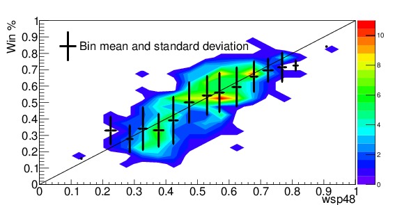
Figure 6. Winning percentage at the end of the season vs combined win shares per 48 minutes at the beginning of the season for all teams from the 1990-1999 seasons. The black points with error bars indicate the means and standard deviations in each of the 20 bins.
E. Evaluating the Predictions
In order to evaluate these methods and the predictions they give, we must test them with real data. To that end, I have gathered the end-of-year statistics for every team and player since 1980; however, only the years since 1986 are useful for our study because prior to that, the statistics I have obtained (from Basketball-Reference.com) do not contain offensive rebounding stats, and some lack field-goal attempts. I have also obtained the game-by-game stats for all players and teams in those seasons. Due to team movement and name changes, a mapping of team names from year to year was created.
i. Compiling the Rosters
Once the data were obtained, it was necessary to compile a roster for each team at the beginning of each season. I was not able to find complete rosters on opening day for all of the teams, so it was generated with the following method. Let’s say I’m looking at the 2014 Philadelphia 76ers. I start by looking through every player who played in the 2014 season. If the player played that season and played only for one team, the 76ers, and he was on the 76ers in the previous season (2013), then he was counted on the team. If he only played for one team, the 76ers, that year, but was not on the team last year, and his first game for the team was during the first month of the season, then he was counted as on the team. The one month cut-off is to try to avoid counting free-agents who may have been added during the course of the season. Clearly, some free-agents and D-league call-ups will be accidentally included, but most will add only marginally to the statistics, because their previous season likely won’t be stellar. If he played for more than one team, but he started with the 76ers and was on the team in their previous season, he was added to the roster. If he was on more than one team, started with the 76ers, but was not on the team last year, then we again require him to play within the first month.
This method does an excellent job of getting everyone who was on the team and able to contribute, and all of the teams whose opening day roster I can confirm independently were correctly generated using this method.
No attempt was made at this time to take into account injuries that would delay the start of a season for a player, but that feature could definitely be added in the future. For instance, it was known that Kevin Durant would miss the first four weeks of the 2015 season due to injury; his stats should be prorated to account for that. That is very difficult to do historically, because you would need to know how long the team thought he would be out at the beginning of the season, not just how long he was actually out. This would be much easier when dealing with the present and future. Nor was any attempt made to consider a young player improving between seasons, nor an older player declining between seasons, though these would be good to implement in the future.
Once the opening-day rosters were assembled, the players stats from the preceding season were added together to get a projected set of statistics. The main stats we are interested in are orp, efgp, ftmr, top, win shares, and minutes played. The rate statistics (orp, efgp, ftmr, and top) are calculated according to their formulas, using for instance the total number of offensive rebounds divided by the total number of offensive-rebounding opportunities; the individual rates themselves are not averaged together in any way.
Players who did not play in the previous season are generally given no stats, even in the case of injury. This could be amended in the future. However, rookies are given a projected amount of win shares and minutes played based on the average amount of production a player chosen in his draft position usually produces. The procedure of figuring out how much to add per draft pick is detailed in Section V. This amount is only added to a team if the player will actually play with the team during the season. Thus, Joel Embiid would not have been added to the 2015 76ers roster as the $latex 3^{rd}$ pick because it was known he was not going to play with the team due to injury, but he would be added to the 2016 76ers team provided he recovers from his injury.
Once all of the rosters have been generated, the means and standard deviations of each of the 9 stats used for the previous year calculations, and the 5 stats used for the current year predictions are tabulated. Please see the Appendix for details of how they are calculated.
ii. Results
Now that I have all of the statistics needed to run the analyses, the weights to be used in each of the distance metrics must be calculated. This process will not be detailed here, but it involves fitting the data for each game in a season using only the 5 or 9 statistics mentioned for each method. Since I do not want to bias the results, I found the weights by fitting the 1990-1999 seasons, and will perform the tests on the 2000-2014 seasons. There were 445 individual team-seasons in this span, however one of those team-seasons was the 2005 expansion Charlotte team, which cannot be analyzed because it did not exist in the previous season and therefore does not have any statistics. That leaves us with 444 seasons to test.
Table II displays the results of the analyses by means of the reduced $latex chi^2$, average absolute value of the difference between the predicted winning percentage and the actual result (this is actually the difference of the percentages times 82 to make it easier to read), and the average standard deviation given by the prediction (again multiplied by 82). Based off of the average differences, it appears that that simply basing the guess for the next season’s results off of the combined win shares on the team at the beginning of the season gives the best results, with the similarity methods not far behind, and the League Average prediction doing worst of all, as expected. However, if we look at the reduced $latex chi^2$ values, it is clear that the similarity methods are making the best predictions of their standard deviations, and they are lower as well. The best method seems to be the Opening-Day-Roster Similarity method, which has a near-perfect $latex chi^2/NDF$, reasonable average difference, and the smallest average standard deviation (other than the Repeat-Last-Year method which vastly under-estimates the standard deviation). It makes sense that the Opening-Day-Roster method is better than the Last-Season version, but it is surprising how well the Last-Season method performs. Perhaps it is a result of teams not making an overwhelming number of changes during the off-season; or it could be that the lack of defensive stats in the Opening-Day-Roster method hurts its performance. This is a good sign, since many decisions on trading draft picks come during the draft, when next year’s roster may not be known. The prediction from win shares alone is very promising as well, and delightful in its simplicity. More work must be done to obtain realistic standard deviations for it though.
| Method | $latex chi^2/NDF$ | $latex 82cdotoverline{|P – p|}$ | $latex 82cdotoverline{sigma_{P}}$ |
| League Average | 0.784 | 10.2 | 13.3 |
| Repeat Last Year | 3.098 | 8.2 | 4.4 |
| Win Shares | 0.737 | 7.1 | 9.4 |
| Similarity Methods | |||
| Last Season | 1.091 | 7.9 | 9.4 |
| Opening-Day Roster | 1.020 | 7.5 | 8.6 |
Table II. The results of each of the six different prediction methods developedin this section. The $latex chi^2/NDF$ indicates how well the errors are estimated compared to the differences seen. The average of the absolute value of the difference between the predicted, P, and actual winning percentage, p, is also given (scaled by 82 to represent number of games), along with the average standard deviation (also in games). As expected, the League Average prediction has the worst results. Repeating last year’s win total performs better in terms of the average differential, but is severely under-estimating the standard deviation. The Win Shares method produces the smallest average differential, but is over-estimating its standard deviation. All of the Similarity methods produce excellent $latex chi^2/NDF$ results, and the Opening-Day-Roster method gives the overall best results.
VII. Putting It All Together: Evaluating Draft Picks in Trades
We’ve finally gotten to a point where we can actually evaluate a potential draft pick from a given team. We will start by looking at the projected finishing-order and draft-order probabilities calculated using Equation (4) along with predictions given by one of the methods described earlier, the Opening-Day-Roster Similarity method. I have selected 3 teams from the 2014 season, and made predictions using that method and then plotted the probabilities for where each team will finish and draft. I tried to select one team predicted to do poorly, another predicted to be in the middle, and one that was likely in the playoffs. The results of these predictions can be seen Figure 7.
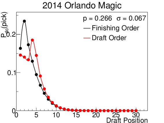
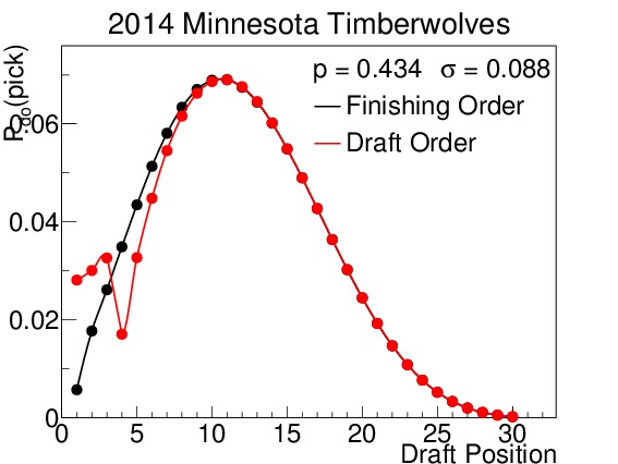
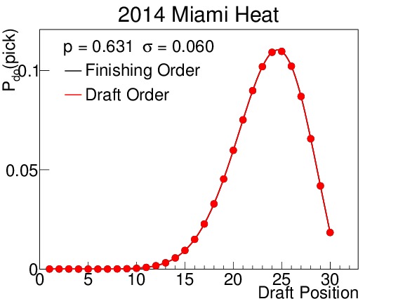
The 2014 Orlando Magic were predicted to finish in the bottom third of the league, and with a maximum likelihood of drafting fourth. In fact they did draft fourth. The 2014 Minnesota Timberwolves were projected to be a classic middle-of-the-road team, with non-zero probabilities of finishing in all but the best two positions in the league. As such, their drafting position is widely varied. Table III displays their odds for picking in each position in both rounds. Note that the odds above pick 14 do not change between rounds because the lottery effects do not come into play. Finally, the 2014 Miami Heat were predicted to finish in the top third of the league, and therefore are almost completely unaffected by the lottery. This prediction correctly forecast their actual drafting position.
(a)
(b)
(c)
Figure 7. $latex mathcal{P}_{do}(delta)$ for all 30 draft positions for (a) the 2014 Orlando Magic, (b) the 2014 Minnesota Timberwolves, and (c) the Miami Heat. Predictions were made using the Opening-Day-Roster Similarity method. Orlando is an example of a team that was projected to do poorly, finish in the second to last spot, and pick fourth; in fact they finished third from last, but did pick in the fourth spot. Minnesota was a great example of a team projected to be in the middle of the pack; they had a non-zero probability of finishing in all but the $latex 29^{th}$ and $latex 30^{th}$ spots. The pick-by-pick probabilities for Minnesota can be seen in Table III. And the Miami team is a good example of a projected playoff team, with almost no probability of finishing in the lottery.
| $latex delta$ | $latex 1^{st}$ Round | $latex 2^{nd}$ Round | Pick | $latex 1^{st}$ Round | $latex 2^{nd}$ Round |
| 1 | 0.006 | 0.028 | 16 | 0.049 | 0.049 |
| 2 | 0.018 | 0.030 | 17 | 0.043 | 0.043 |
| 3 | 0.026 | 0.033 | 18 | 0.036 | 0.036 |
| 4 | 0.035 | 0.017 | 19 | 0.030 | 0.030 |
| 5 | 0.043 | 0.033 | 20 | 0.024 | 0.024 |
| 6 | 0.051 | 0.045 | 21 | 0.019 | 0.019 |
| 7 | 0.058 | 0.055 | 22 | 0.015 | 0.015 |
| 8 | 0.063 | 0.062 | 23 | 0.011 | 0.011 |
| 9 | 0.067 | 0.066 | 24 | 0.008 | 0.008 |
| 10 | 0.069 | 0.069 | 25 | 0.005 | 0.005 |
| 11 | 0.069 | 0.069 | 26 | 0.003 | 0.003 |
| 12 | 0.067 | 0.068 | 27 | 0.002 | 0.002 |
| 13 | 0.064 | 0.065 | 28 | 0.001 | 0.001 |
| 14 | 0.060 | 0.060 | 29 | 0.000 | 0.000 |
| 15 | 0.055 | 0.055 | 30 | 0.000 | 0.000 |
Table III. $latex mathcal{P}_{do}(delta)$ for each round for the 2014 Minnesota Timberwolves based off of the prediction made using the Opening-Day-Roster Similarity method. The $latex 1^{st}$-round odds take the lottery effects into account, while the $latex 2^{nd}$-round odds are based solely on finishing order.
A. Expectation Values
When considering a draft pick in trade, it is sometimes useful just to think of where the pick is most likely to fall (i.e. which spot has the highest probability), and other times it is useful to think of the probabilities of certain ranges where that pick could fall. If a draft pick is offered with certain protections, say top-5 protected, then the probability that the pick will fall inside or outside of the top 5 picks is important. In that case, all one has to do is to sum the probabilities of each spot up for the two categories. Thus, the odds of the 2014 Minnesota Timberwolves picking inside the top 5 are 0.006 + 0.018 + 0.026 + 0.035 + 0.043 = 0.128, while their odds of picking outside the top 5 are 1 – 0.128 = 0.872.
We can also consider the expectation value for the picks, where the expectation value is defined as the weighted average of the possible draft order positions, $latex delta$, given a prediction percentage $latex P,sigma_P$, and is written as
$latex <delta|P,sigma_P> = frac{sumlimits_{delta} (mathcal{P}(delta|P,sigma_P)cdot delta)}{sumlimits_{delta}mathcal{P}(delta|P,sigma_P)}~,hfill (16) &s=2$
where the sums are over all non-protected picks. If we look at the 2014 Timberwolves again, we can calculate their overall expectation value to be 11.7 (sum over all $latex delta$) however, if this pick was offered in a trade, with the first 5 picks protected, then the expectation value of the pick that would be received would only be 12.9 (sum over $latex delta geq 6$). As can be seen from the graph of their drafting probabilities, this is right at the position of their most likely draft slot.
B. Expected Return
Say a team is considering trading away a player who is forecast to generate about 10 win shares over the next 5 years, and they would like to upgrade to a player who should produce at least 12.5 win shares during that time. They are offered trades by both Minnesota and Orlando, who are offering their 2014 first-round draft pick just before the 2014 season starts. Both are top-3 protected. Which team should they trade with?
To evaluate the values of the two offers they need to have a prediction for how well each of them will do in the upcoming season. So they use the Opening-Day-Roster Similarity method to generate a prediction, and figure out the odds for each team getting each draft slot, which we have already seen. Now, we modify our expectation value formula slightly, by replacing the pick with win shares to get the expected return (in win shares) from the pick:
$latex <ws|P,sigma_P> = frac{sumlimits_{delta} (mathcal{P}(delta|P,sigma_P)cdot ws(delta))}{sumlimits_{delta}mathcal{P}(delta|P,sigma_P)}~, hfill (17) &s=2$
where the number of predicted win shares is a function of the position in which the player was drafted, $latex delta$, derived in Section V. They must still remember that each trade has protected certain slots, and so they also need the probability of getting each team’s spot due to the protection; this is just the denominator in Equation (17). Working the numbers through, we see that Minnesota’s draft pick has an expectation value of 11.53 win shares over the next 5 years, and has a 90.9% chance of being outside of the top 3; the upgrade is less than desired, but it is very likely that the pick will actually be transferred to the team in the next draft. Orlando’s pick meanwhile is likely to be worth 18.75 win shares over the next 5 years, a much bigger upgrade than expected, but with only a 56.5% chance of getting it this draft.
Which trade to choose in this situation can depend on many factors, such as how quickly the team needs a return on the trade, how willing the GM and owner are to gamble, what the terms are if the draft pick ends up being protected, etc. But knowing the expected return and probability of receiving the pick in the nearest draft allows them to make an informed decision.
VIII. Conclusion
The goal of this exercise was to find a way to put a value on draft picks offered in trade. Equation (17) does just that, providing an expected return, in terms of win shares over the player’s first five seasons, from an offered draft pick based on a prediction for the team’s performance in the coming year, and taking into account any protections placed on the pick. Using this formula, it is easy to make a comparison between two competing offers, as well as between the draft pick and the asset being traded. Of course, the statistic that an expected return is calculated for in Equation (17) can be replaced with any other statistic, all it requires is a way to calculate an prediction for that statistic as a function of draft position. Thus, the expected return in minutes played could be calculated based on the analysis presented in this paper, but so can rebounds, points, or any other statistic.
The prediction for expected return is only as good as the predictions for winning percentage and standard deviation are. I have developed three methods that yield consistent results, the two Similarity methods and the forecast directly from win shares, and other methods may be developed. Fortunately, any prediction can be fed into Equation (17), so any improvements to the current methods, or brand-new methods developed can immediately be turned into an expected return, and various methods can be used for comparison purposes.
A. Future Work: Improvements
Each and every step along the way can benefit from more work, and there is room for improvement in many areas, some of which have already been mentioned. I have shown that there is a slight difference between playoff probabilities in the Eastern and Western Conferences; an early attempt to correct for this was not successful, so it would be good to revisit this issue and figure out a way to increase the odds that a Western Conference team with 40-50 wins will be relegated to the lottery.
Valuing the draft picks was done using only win shares and minutes played in the first five seasons of a player’s career in this paper. As has been mentioned, many other stats could be used in the place of win shares. Several stats could be treated individually, or a function could be generated to create a new statistic out of those several stats. And the number of years considered in these stats can be easily changed as well.
The way of predicting a team’s winning percentage can always be improved upon. I mentioned various tweaks to some of the methods in Section VI. Some of the easiest tweaks would be to include more than just the previous season’s stats in the methods, accounting for injuries in the previous season by using another season instead, updating the predictions throughout the season based on roster changes as well as adding in the current season’s results, and developing a way to account for defense in the the Opening-Day-Roster similarity method. Others include obtaining the complete roster, along with any injury reports, for each team for every day of the year historically (necessary to improve the models); finding the best set of statistics to use in the similarity metrics; making predictions for rookies performance in the four factors to improve the Opening-Day-Roster similarity method; and modeling improvements in stats for young players, and declining stats for older players to improve the accuracy of the roster stats.
Trying to incorporate coaching, or at least coaching style, into the predictions would be a fertile area for improvement. The difficulty here is trying to disentangle a coach’s impact on his team from the players themselves, as well as dealing with first-year coaches, coaches on a new team, etc. There is much value to be gained from looking into the coaches contributions.
In this paper, I only looked at predicting the immediate next season, but since draft picks can be traded up to seven years in advance, it may be necessary to predict teams’ fortunes even further than just next season. It is of course possible to do this, though the standard deviations will only get larger as the years get further away.
For the final prediction, of expected return from the proposed trade, a variety of other statistics could be used. The expected salary that will need to be payed out to a prospective pick can be nearly exactly calculated from the known rookie scale, and would be an easy addition to make.
Finally, I have specifically avoided calculating the standard deviation of the expected return because it is a complicated value. The value
$latex sigma_{<wp>} = sqrt{<wp^2> – <wp>^2} hfill (18) &s=2$
gives the standard deviation of the average expected return value for that pick, but the errors on that average in any given slot can be as many as 15 win shares (see Figure 5). Thus, citing a standard deviation of 3.1 win shares for Orlando’s pick would make it seem much smaller than the actual uncertainty. Coming up with a way to display both uncertainties in the future would be helpful.
Appendix:
Calculating Standard Deviations of Rate Statistics with an Unequal Number of Opportunities
The standard deviation of a dataset is a well-defined quantity (I will square both sides to avoid the constant square-root sign)
$latex sigma^2 = frac{1}{N-1}sumlimits_{i=1}^N(p_i – bar{p})^2~, hfill(A1) &s=2$
where $latex bar{p}$ is the mean of the dataset. However, that assumes that each term should be treated equally. Since the standard deviation on rate statistics depends on the number of opportunities, and players and teams in basketball can have wildly varying numbers of opportunities with respect to each other over the course of a season, it makes sense to weight certain terms more than others. Equation (A1) can then be generalized to
$latex sigma^2 = frac{1}{sumlimits_{i=1}^N frac{1}{sigma_{i}^2}}sumlimits_{i=1}^N frac{1}{sigma_{i}^2} (p_i – bar{p})^2~, hfill (A2) &s=2$
where the weights are determined to be the inverse of the square of the standard deviation of the term, defined by Equation (5).
Let us take the three-point shooting percentage as an example. Consider the five Atlantic division teams in 2014 with the following statistics (threem, threea): [BOS (575,1729), BRK (709,1922), NYK (759,2038), PHI (577,1847), TOR (713,1917)]. The mean shooting percentage is just
$latex overline{threep} = frac{sumlimits_i threem_i}{sumlimits_i threea_i} = 0.353~. hfill (A3) &s=2$
The traditional standard deviation is 0.028, while the weighted standard deviation is 0.025. In this example the Knick’s 2038 attempts are nearly 18% more than Boston’s 1729, and so their measured value carries more weight than Boston’s as well. The difference may seem slight, but it can make a significant difference. Plotting the distributions with the same weights makes them appear more Gaussian than without the weights, and as a result, the Gaussian approximation better.
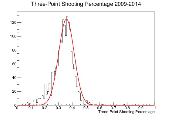
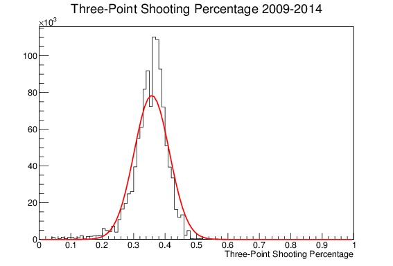
To illustrate that point, consider the plots of three-point shooting percentages I made for my project on regression to the mean, which can be seen in Figure 8. It shows the end-of-the-year three-point shooting percentages for all players in the NBA in the 2009-2014 season. Figure (a) is unweighted and shows a noticeable tail on the lower edge of the distribution, and is poorly fit by a Gaussian with parameters set to its mean and traditional standard deviation. Figure (b) meanwhile shows the same distribution, but this time with each term weighted by its standard deviation. The tail on the low edge is greatly reduced, because the players shooting at a lower percentage tend to shoot less. The Gaussian approximation, using the mean and weighted standard deviation as parameters, is a much better fit.
(a)
(b)
Figure 8. End-of-the-year Three-point Shooting Percentages for all players in the NBA from 2009-2014, along with a Gaussian approximation fit line using the calculated mean and weighted standard deviation. (a) shows the unweighted distribution, which has a tail on the lower edge, and is not well fit by the Gaussian. (b) shows the same distribution where each entry is weighted by its standard deviation; the lower edge tail is gone and the Gaussian is a much better approximation for the shape.